〇、说明 使用scipy库来设计低通滤波器,这里使用1Hz与50Hz的两个频率信号叠加,之后通过滤波器之后观察效果。
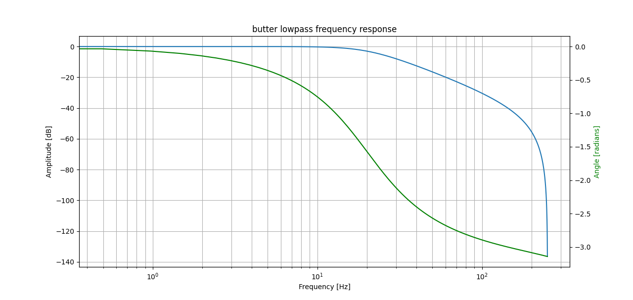
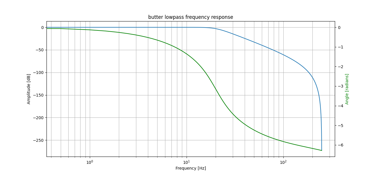
一、滤波器设计 使用signal.sosfreqz得到幅频响应。
1 2 3 4 5 6 7 8 9 10 11 12 13 14 15 16 17 18 19 sos=signal.butter(2 , 20 , 'lowpass' , fs=500 , output='sos' ) w, h = signal.sosfreqz(sos, fs=500 ) fig = plt.figure() ax = fig.add_subplot(1 , 1 , 1 ) ax.semilogx(w, 20 * np.log10(abs (h))) ax.set_title('butter lowpass frequency response' ) ax.set_xlabel('Frequency [Hz]' ) ax.set_ylabel('Amplitude [dB]' ) ax.grid(which='both' , axis='both' ) ax2 = ax.twinx() angles = np.unwrap(np.angle(h)) ax2.plot(w, angles, 'g' ) ax2.set_ylabel('Angle [radians]' , color='g' ) plt.show()
程序的图形如下:
二、滤波效果 1 2 3 4 5 6 7 8 9 10 11 12 13 14 15 16 17 18 19 20 21 22 23 24 25 26 27 28 29 30 31 32 33 34 35 36 37 38 39 40 41 42 43 44 45 46 47 48 49 50 51 52 53 54 55 56 57 58 59 60 61 62 63 64 65 66 67 68 69 70 71 72 73 74 75 76 77 from scipy import signalimport numpy as npimport matplotlib.pyplot as pltfrom scipy.fft import fftfreqN=500 T=1 /N t = np.linspace(0 , T*N, N, False ) sig1=np.sin(2 *np.pi*1 *t) sig2=np.sin(2 *np.pi*50 *t) sig = sig1 + sig2 fig, (ax1, ax2,ax3) = plt.subplots(3 , 1 , sharex=True ) ax1.plot(t, sig) ax1.set_title('10 Hz and 50 Hz sinusoids' ) ax1.axis([0 , T*N, -2 , 2 ]) ax1.grid() sos = signal.butter(2 , 20 , 'lp' , fs=N, output='sos' ) filtered = signal.sosfilt(sos, sig) ax2.plot(t, filtered) ax2.set_title('After 15 Hz lp-pass filter' ) ax2.axis([0 , T*N, -2 , 2 ]) ax2.set_xlabel('Time' ) ax2.grid() plt.tight_layout() b,a=signal.sos2tf(sos) b0=b[0 ] b1=b[1 ] b2=b[2 ] a0=a[0 ] a1=a[1 ] a2=a[2 ] def filr2 (data ): out=[] Xn1 = 0 Xn2 = 0 Yn1 = 0 Yn2 = 0 index=0 sample=len (data) while sample > 0 : Xn = data[index] acc = (b0 * Xn) + (b1 * Xn1) + (b2 * Xn2) -(a1 * Yn1) - (a2 * Yn2) out.append(acc) Xn2 = Xn1 Xn1 = Xn Yn2 = Yn1 Yn1 = acc index+=1 sample-=1 return out out=filr2(sig) ax3.plot(t, out) ax3.set_title('After 15 Hz low-pass filter' ) ax3.axis([0 , T*N, -2 , 2 ]) ax3.set_xlabel('Time' ) plt.tight_layout() ax3.grid() plt.show()
signal.sosfilt可以参考官方文档 ,或者该中文示例 。
频谱的计算与显示:
1
2
3
4
5
6
7
8
9
10
def amp_ang_resp (data,N,T ): yf= np.fft.fft(data) xf = fftfreq(N, T)[:N//2 ] plt.plot(xf, 2.0 /N * np.abs (yf[0 :N//2 ])) plt.grid() plt.show() amp_ang_resp(sig,N,T) amp_ang_resp(filtered,N,T) amp_ang_resp(out,N,T)
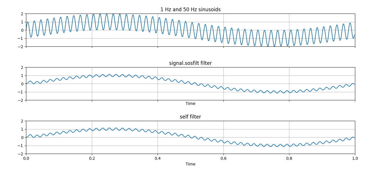
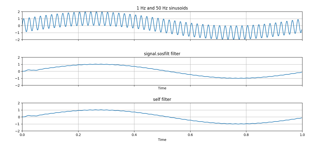
1、采样率N=500 (1)原始数据的波形与使用两种方法滤波后的波形。
从上图可以明显的看出滤波效果,即仍然存在小幅度的比较高的频率信号。
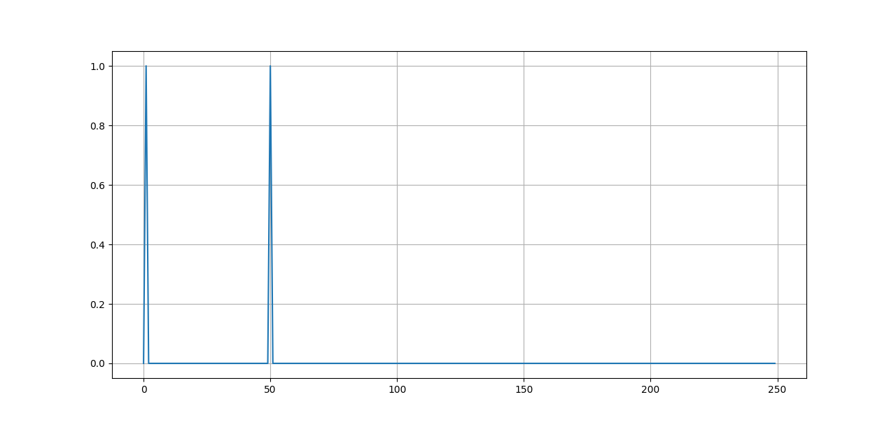
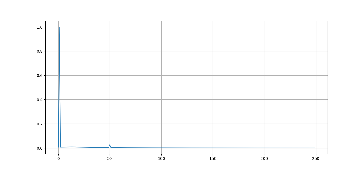
(2)原始数据的频谱:
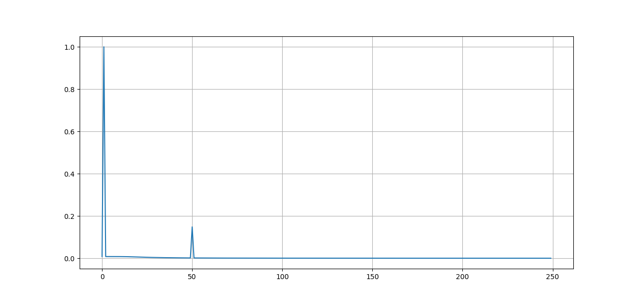
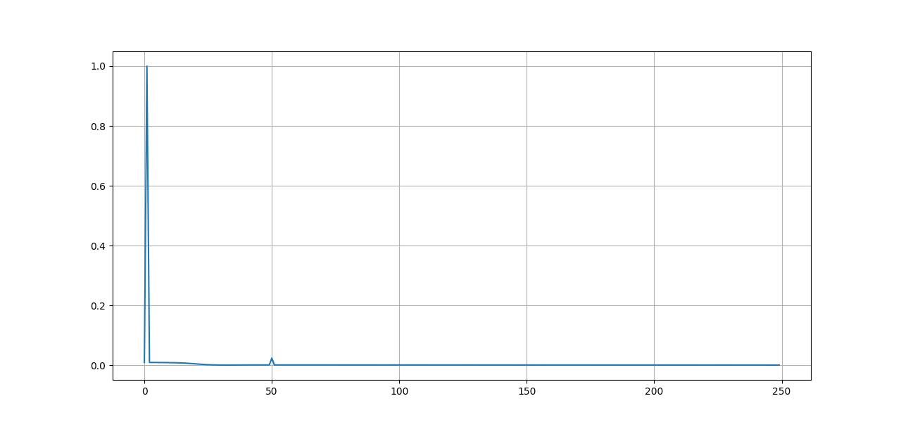
(3)使用signal.sosfilt滤波后的频谱:
(4)使用自己写的函数处理后的频谱:
从频谱图中可以清晰的看到,在50Hz处存在一个小的幅值。
2、增加阶数 (1)如果仍使用上述参数,但是滤波处理函数改为signal.sosfiltfilt,那么效果会变好,但是相当于阶数增加为4阶了。
signal.sosfiltfilt官方文档
Using forward-backward filtering, whether it is using the b,a parameter form or the sos form, doubles the effective order of the filtering when compared to a simple forward filter. That is the reason why scipy.signal.sosfiltfiltsosfiltfilt with an 8th-order Butterworth filter using sosfilt.参考
在其它参数不变的情况下,使用signal.sosfiltfilt滤波的效果如下图所示:
(2)若使用4阶的系数,那么同样效果会比较好,如下图。同时需要做如下修改:
1 sos = signal.butter(4 , 20 , 'lp' , fs=N, output='sos' )
滤波器幅频响应如下:
使用signal.filt的效果:
使用自己写的滤波函数的效果:
4阶的计算方法如下:
1
2
3
4
5
6
7
8
9
10
11
12
13
14
15
16
17
18
19
20
21
22
23
24
25
26
27
28
29
30
31
32
33
34
35
36
37
38
39
40
41
42
43
44
45
46
47
48
49
b,a=signal.sos2tf(sos) b0=b[0 ] b1=b[1 ] b2=b[2 ] b3=b[3 ] b4=b[4 ] a0=a[0 ] a1=a[1 ] a2=a[2 ] a3=a[3 ] a4=a[4 ] pState=[0 ,0 ,0 ,0 ,0 ,0 ,0 ,0 ] def filr4 (data ): global pState out=[] Xn1 = pState[0 ]; Xn2 = pState[1 ]; Xn3 = pState[2 ]; Xn4 = pState[3 ]; Yn1 = pState[4 ]; Yn2 = pState[5 ]; Yn3 = pState[6 ]; Yn4 = pState[7 ]; index=0 sample=len (data) while sample > 0 : Xn = data[index] acc = (b0 * Xn) + (b1 * Xn1) + (b2 * Xn2)+ (b3 * Xn3) + (b4 * Xn4) -(a1 * Yn1) - (a2 * Yn2) -(a3 * Yn3) - (a4 * Yn4) out.append(acc) Xn4 = Xn3 Xn3 = Xn2 Xn2 = Xn1 Xn1 = Xn Yn4 = Yn3 Yn3 = Yn2 Yn2 = Yn1 Yn1 = acc index+=1 sample-=1 return out
下面几句话与上面没有太大的关系,但是挺有启发意义,记录下。参考
采样频率是联系离散时间域和连续时间域的纽带:从时域上看,采样频率的倒数代表了两个相邻样点间的时间;从频域上看,采样频率的一半是离散时间信号所能表征的最高频率。
所以,数字滤波器的设计,不管是通带截止频率还是阻带截止频率,理论上都不能超过采样频率的一半。实际上,在数字滤波器设计中,通常把采样频率的一半定义为归一化频率“1”,用一个小于“1”的值(比如说0.2)来定义数字滤波器的通带或阻带截止频率(相当于定义的是截止频率对半采样率的比值)。
工程上,在较高采样率上实现数字滤波器,一般而言功耗会大一些。但在过低的采样率上实现数字滤波器也会有一些实际的限制:想象一下,如果要实现一个归一化截止频率为0.49的低通滤波器,会要求多窄的滤波器过度带(0.49~0.5);而只要采样率升高一倍,相同低通滤波器的归一化截止频率就变成了0.245,就不会有实现上的困难了。